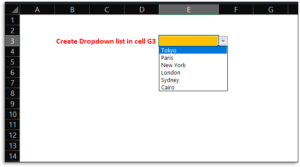
Hey Datalunatics, if you want to add a dropdown list in an Excel sheet quickly then you are at the right post. I will help you to add a dropdown list in a step-by-step guide. Let’s start with it.
First of all, you will need a list that you want to add in a dropdown. I have taken an example below of which we will create a dropdown list. You can follow the same steps.
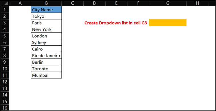
In the above picture, we have city names in the B column and we want to create a dropdown list on City Names in G3 Cell. Your scenario can be different in terms of the address of the dropdown list cell but the process is similar.
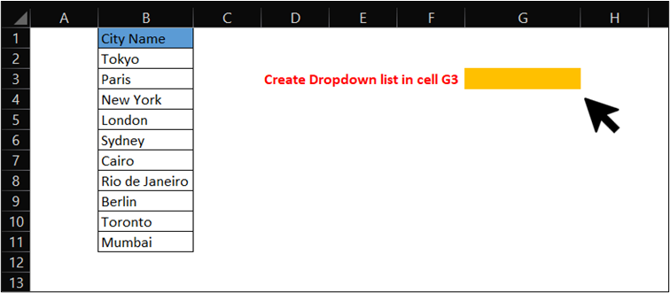
Now select the cell where you want to apply the dropdown list, In our scenario, I have selected the cell G3.
Now, Go to the “Data” tab and click on the “Data Validation” option, you will get a dialog box as shown below.
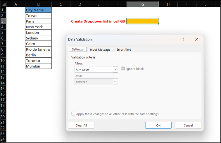
Now, In the “Settings” tab, select “List” in the “Allow:” option as shown below.
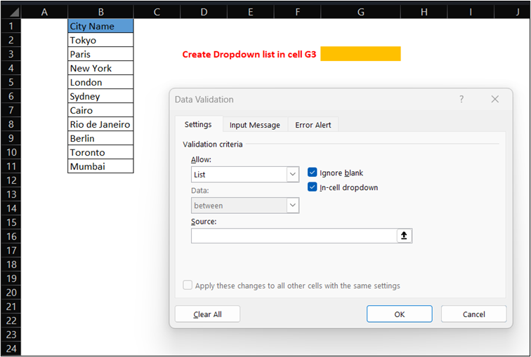
Now, In the “Source” criteria, Select the cell range that you want to add to the dropdown list. I have selected the B2:B11 cell range.
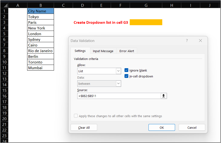
Click “OK” to apply and you can see the dropdown list is added in cell G3.
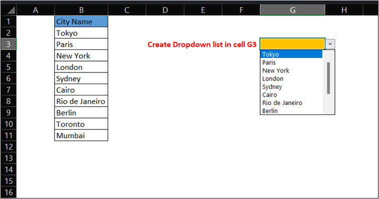
Add Criteria in the Dropdown List Manually:
So, we have added the dropdown list successfully. But sometimes, you may have a scenario where you don’t have a cell range of City Names as we have in Column B and if you want to add city Names manually without any cell range then you can add that as well. Let’s see how we can do that.
Go to the “Data” tab and Click on “Data Validation” option. Now we can enter the names of city manually in Source criteria.
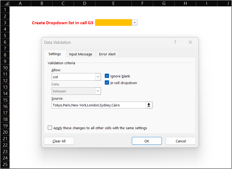
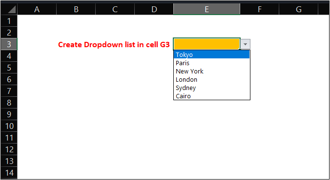
In the above picture, we can see that we have added City Names in the Source criteria Manually (Which are : Tokyo,Paris,New York,London,Sydney,Cairo) and This will create the dropdown list for these cities’ names as shown below.
How to add a dynamic dropdown list:
Now, you can make your dropdown list dynamic which means whenever you add any name in your criteria range it should automatically reflect in your dropdown list. We have a similar City name in column B that we want to add to a dropdown list.
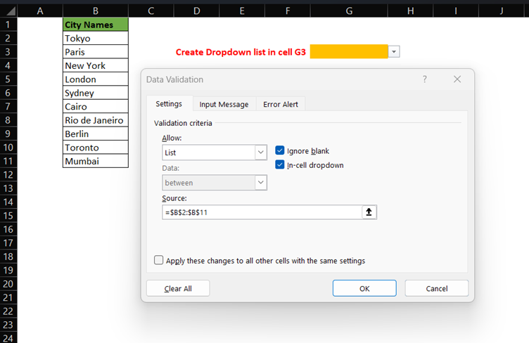
We have selected the cell range only from B2 to B11 but when we add any city below Mumbai it will not add that name in the dropdown list as we have entered a fixed range in the criteria and to make the range dynamic we have to follow the below steps.
First Convert the Cell range into Table format. To convert the cell range into a Table, go to the “Insert” tab and click on the “Table” Option.
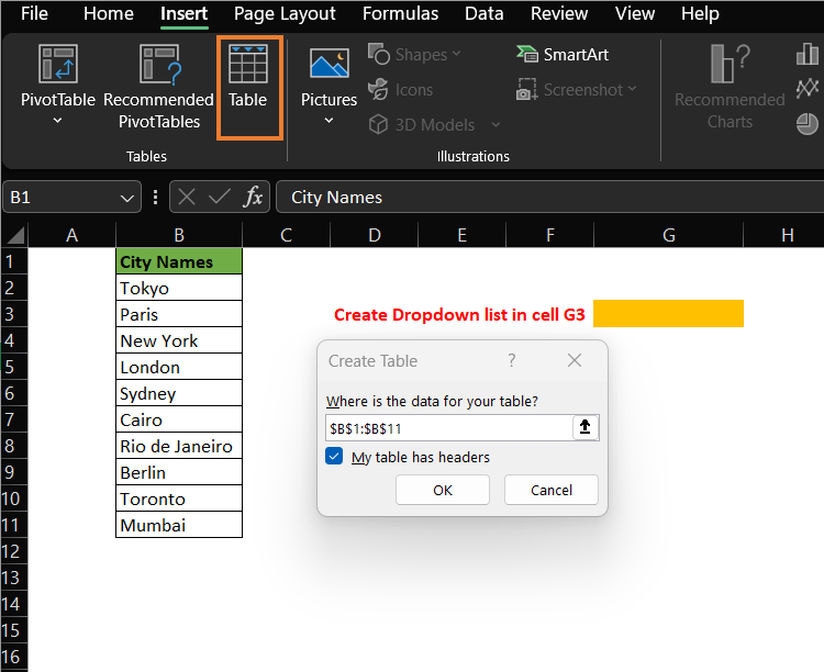
The range would be selected automatically and click on “OK” to convert the selected range in the Table.
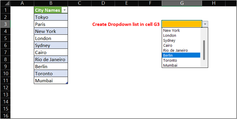
In the above picture, we have converted the cell range into a Table and you can see that in the Dropdown list, Mumbai is the last name. Let’s add a new city name in the B column as “Barcelona”
You will see that the “Barcelona” city name is automatically added to the dropdown list.
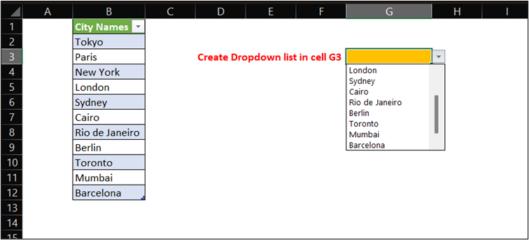
So, by following these steps, you can create a dynamic dropdown list.
Conclusion:
We have seen the step-by-step guide to add the dropdown list in Excel. Hope this can help you to add the Dropdown list. Please let me know in the comments about any Excel trick you want to share. I will see you in another post.

